Show the code
pacman::p_load(jsonlite, tidygraph, ggraph,
               visNetwork, graphlayouts,
skimr, tidytext, tidyverse)FishEye International, a non-profit focused on countering illegal, unreported, and unregulated (IUU) fishing, has been given access to an international finance corporation’s database on fishing related companies. In the past, FishEye has determined that companies with anomalous structures are far more likely to be involved in IUU (or other “fishy” business). FishEye has transformed the database into a knowledge graph. It includes information about companies, owners, workers, and financial status. FishEye is aiming to use this graph to identify anomalies that could indicate a company is involved in IUU.
FishEye analysts have attempted to use traditional node-link visualizations and standard graph analyses, but these were found to be ineffective because the scale and detail in the data can obscure a business’s true structure. Can you help FishEye develop a new visual analytics approach to better understand fishing business anomalies?
Use visual analytics to understand patterns of groups in the knowledge graph and highlight anomalous groups.
Use visual analytics to identify anomalies in the business groups present in the knowledge graph. Limit your response to 400 words and 5 images.
Develop a visual analytics process to find similar businesses and group them. This analysis should focus on a business’s most important features and present those features clearly to the user. Limit your response to 400 words and 5 images.
Measure similarity of businesses that you group in the previous question. Express confidence in your groupings visually. Limit your response to 400 words and 4 images.
Based on your visualizations, provide evidence for or against the case that anomalous companies are involved in illegal fishing. Which business groups should FishEye investigate further? Limit your response to 600 words and 6 images.
In this exercise, only question 1 and question 2 would be explored.
pacman::p_load(jsonlite, tidygraph, ggraph,
visNetwork, graphlayouts,
skimr, tidytext, tidyverse)mc3 <- jsonlite::fromJSON("data/MC3.json")#view(mc2[["nodes"]])
mc3_nodes <- as_tibble(mc3$nodes) %>%
mutate(country=as.character(country),
id=as.character(id),
product_services=as.character(product_services),
revenue_omu = as.numeric(as.character(revenue_omu)),
type=as.character(type)) %>%
select(id,country, type, revenue_omu, product_services)
# group_by(id,country, type, product_services) %>%
# summarise(count=n(),revenue=sum(revenue_omu))skim(mc3_nodes)| Name | mc3_nodes |
| Number of rows | 27622 |
| Number of columns | 5 |
| _______________________ | |
| Column type frequency: | |
| character | 4 |
| numeric | 1 |
| ________________________ | |
| Group variables | None |
Variable type: character
| skim_variable | n_missing | complete_rate | min | max | empty | n_unique | whitespace |
|---|---|---|---|---|---|---|---|
| id | 0 | 1 | 6 | 64 | 0 | 22929 | 0 |
| country | 0 | 1 | 2 | 15 | 0 | 100 | 0 |
| type | 0 | 1 | 7 | 16 | 0 | 3 | 0 |
| product_services | 0 | 1 | 4 | 1737 | 0 | 3244 | 0 |
Variable type: numeric
| skim_variable | n_missing | complete_rate | mean | sd | p0 | p25 | p50 | p75 | p100 | hist |
|---|---|---|---|---|---|---|---|---|---|---|
| revenue_omu | 21515 | 0.22 | 1822155 | 18184433 | 3652.23 | 7676.36 | 16210.68 | 48327.66 | 310612303 | ▇▁▁▁▁ |
#view(mc2[["links"]])
mc3_edges <- as_tibble(mc3$links) %>%
  distinct() %>%
  mutate(source=as.character(source),
         target=as.character(target),
         type=as.character(type)) %>%
  mutate(source=as.character(source)) %>%
  group_by(source, target, type) %>%
  summarise(weight=n()) %>%
  filter(source!=target) %>%
ungroup()mc3_edges <- rbind(mc3_edges %>%
mutate(source = ifelse(grepl("^c\\(.*\\)$", source), source, NA)) %>%
drop_na() %>%
mutate(source = strsplit(gsub("^c\\(\"|\"\\)$|\"", "", source), ",\\s*")) %>%
unnest(source),
mc3_edges[!grepl("^c\\(.*\\)$", mc3_edges$source), ])skim(mc3_edges)| Name | mc3_edges |
| Number of rows | 27169 |
| Number of columns | 4 |
| _______________________ | |
| Column type frequency: | |
| character | 3 |
| numeric | 1 |
| ________________________ | |
| Group variables | None |
Variable type: character
| skim_variable | n_missing | complete_rate | min | max | empty | n_unique | whitespace |
|---|---|---|---|---|---|---|---|
| source | 0 | 1 | 6 | 64 | 0 | 13158 | 0 |
| target | 0 | 1 | 6 | 28 | 0 | 21265 | 0 |
| type | 0 | 1 | 16 | 16 | 0 | 2 | 0 |
Variable type: numeric
| skim_variable | n_missing | complete_rate | mean | sd | p0 | p25 | p50 | p75 | p100 | hist |
|---|---|---|---|---|---|---|---|---|---|---|
| weight | 0 | 1 | 1 | 0 | 1 | 1 | 1 | 1 | 1 | ▁▁▇▁▁ |
There are plenty of rows in “source” column are comma separated characters, I broke them into individual rows by deliminator of “,”, remove all those “c(”“)”, and then rebind with other normal columns.
mc3_edges %>%
  group_by(type) %>%
  summarise(count=n())
# A tibble: 2 × 2
type count
<chr> <int>
1 Beneficial Owner 18691
2 Company Contacts 8478product_check <- left_join(mc3_nodes %>%
group_by(type) %>%
summarise(nodes=n()),
mc3_nodes %>%
mutate(n_0 = str_count(product_services, "character")) %>%
filter(n_0>0) %>%
group_by(type) %>%
summarise(empty_product=n()),
by=join_by(type),
keep=FALSE)%>%
mutate(nodes_with_product=nodes-empty_product)
product_check# A tibble: 3 × 4
type nodes empty_product nodes_with_product
<chr> <int> <int> <int>
1 Beneficial Owner 11949 11926 23
2 Company 8639 1 8638
3 Company Contacts 7034 7033 1Most of Beneficial Owner and Company Contacts nodes’ product_services are indicated as “character(0)”, so only “Company” type of nodes got specific product and services description.
company_contacts <- mc3_nodes%>%
  select(id,type) %>%
  filter(type=='Company') %>%
  distinct() %>%
  inner_join(mc3_edges%>%
              filter(type=='Company Contacts'),
            by=join_by(id==source),
            keep=TRUE,
            multiple="all",
            suffix=c('_nodes','_edges')) %>%
  group_by(source,target) %>%
  summarise(weight=sum(weight)) %>%
  arrange(desc(weight)) %>%
ungroup()top10_contacts<- pull(head(company_contacts %>%
group_by(source) %>%
summarise(count=n(),weight=sum(weight)) %>%
arrange(desc(count)), 10),source)
ggplot(data = company_contacts %>%
group_by(source) %>%
summarise(count=n(), weight=sum(weight)) %>%
arrange(desc(count)) %>%
head(10),
aes(x = reorder(source, weight),y=weight)) +
geom_col()+
xlab(NULL) +
coord_flip() +
labs(x = "Company",
y = "Weight",
title = "Top 10 Companies with most company contacts")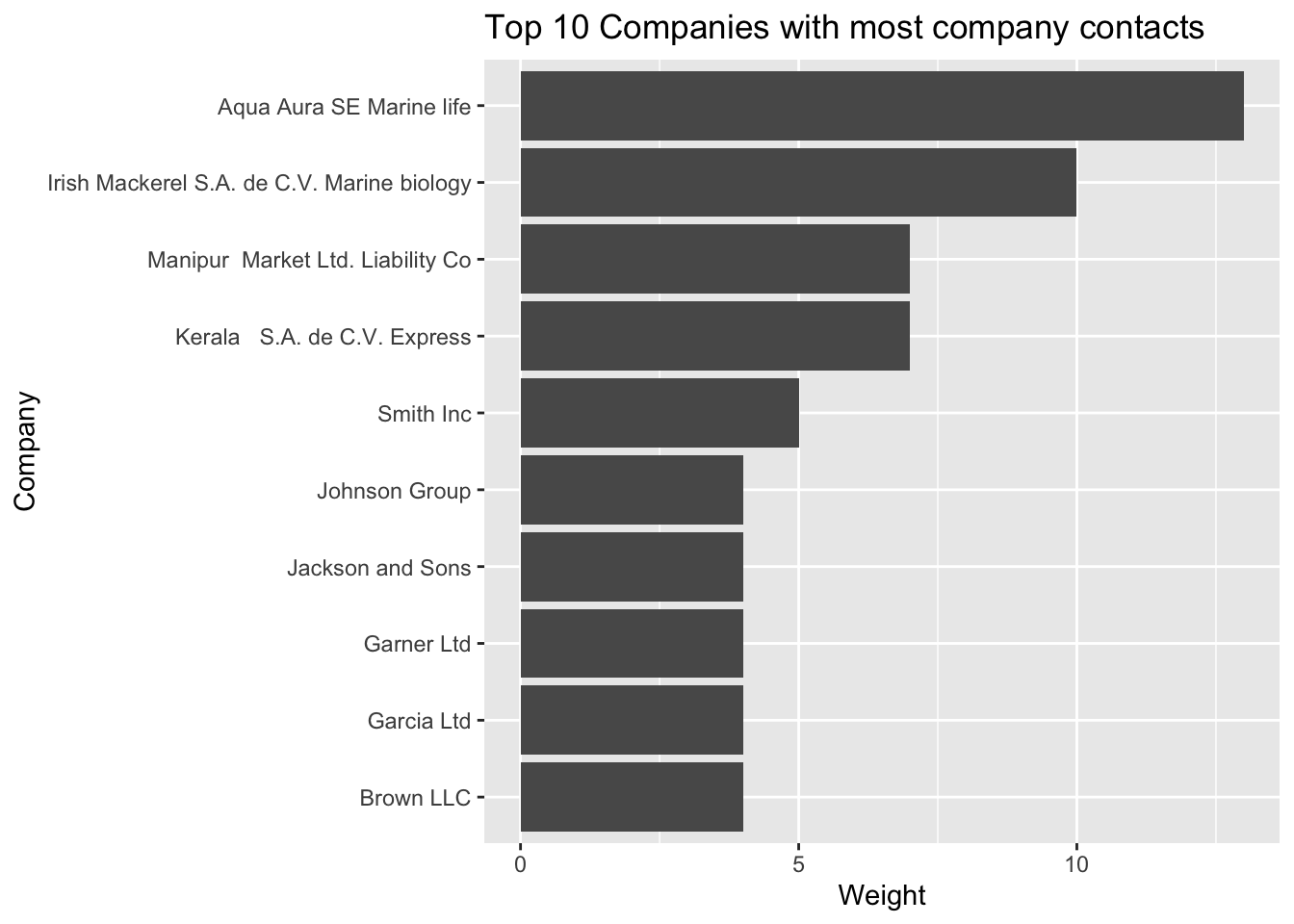
edges1 <- mc3_edges %>%
  filter(grepl(top10_contacts[1],source)) %>%
  group_by(source,target,type) %>%
  summarise(weight=sum(weight)) %>%
  drop_na(weight) %>%
ungroup()nodes1_extract <- rbind(edges1 %>%
rename(id=source)%>%
mutate(group='company') %>%
select(id,group)%>%
distinct(),
edges1 %>%
rename(id=target) %>%
rename(group=type) %>%
select(id,group) %>%
distinct())nodes1_extract%>%
group_by(id) %>%
summarise(count=n())%>%
filter(count>1)# A tibble: 0 × 2
# ℹ 2 variables: id <chr>, count <int>graph1 <- tbl_graph(nodes = nodes1_extract,
edges = edges1,
directed = FALSE) %>%
mutate(between = centrality_betweenness(),
close = centrality_closeness(),
degree = centrality_degree())graph1 %>%
ggraph(layout = "fr") +
geom_edge_link(aes(width=weight,color=type),
alpha=0.8) +
scale_edge_width(range = c(0.5,3)) +
geom_node_point(aes(alpha=0.5,
size = degree,
color = group)) +
scale_size_continuous(range=c(1,5))+
geom_node_text(aes(filter=degree >= 3, label=id), show.legend = FALSE, size=4) +
theme_graph()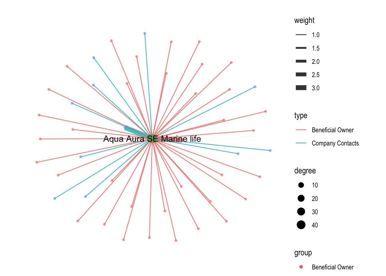
edges2 <- mc3_edges %>%
  filter(grepl(top10_contacts[2],source)) %>%
  group_by(source,target,type) %>%
  summarise(weight=sum(weight)) %>%
  drop_na(weight) %>%
ungroup()nodes2_extract <- rbind(edges2 %>%
rename(id=source)%>%
mutate(group='company') %>%
select(id,group)%>%
distinct(),
edges2 %>%
rename(id=target) %>%
rename(group=type) %>%
select(id,group) %>%
distinct())graph2 <- tbl_graph(nodes = nodes2_extract,
edges = edges2,
directed = FALSE) %>%
mutate(between = centrality_betweenness(),
close = centrality_closeness(),
degree = centrality_degree())graph2 %>%
ggraph(layout = "fr") +
geom_edge_link(aes(width=weight,color=type)) +
scale_edge_width(range = c(0.5,3)) +
geom_node_point(aes(size = degree,
color = group)) +
scale_size_continuous(range=c(1,5))+
geom_node_text(aes(filter=degree >= 3, label=id), show.legend = FALSE, size=4) +
theme_graph()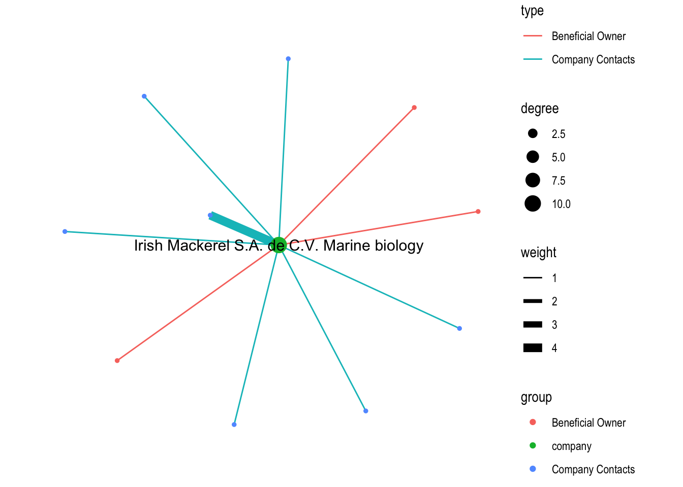
Here we can see an abnormal network in which most of edges are connected with it’s company contacts, and the edge with highest weight is connected with it’s company contracts.
edges3 <- mc3_edges %>%
  filter(grepl(top10_contacts[3],source)) %>%
  group_by(source,target,type) %>%
  summarise(weight=sum(weight)) %>%
  drop_na(weight) %>%
ungroup()nodes3_extract <- rbind(edges3 %>%
rename(id=source)%>%
mutate(group='company') %>%
select(id,group)%>%
distinct(),
edges3 %>%
rename(id=target) %>%
rename(group=type) %>%
select(id,group) %>%
distinct())graph3 <- tbl_graph(nodes = nodes3_extract,
edges = edges3,
directed = FALSE) %>%
mutate(between = centrality_betweenness(),
close = centrality_closeness(),
degree = centrality_degree())graph3 %>%
ggraph(layout = "kk") +
geom_edge_link(aes(width=weight,color=type)) +
scale_edge_width(range = c(0.5,3)) +
geom_node_point(aes(size = degree,
color = group)) +
scale_size_continuous(range=c(1,5))+
geom_node_text(aes(filter=degree >= 3, label=id), show.legend = FALSE, size=4) +
theme_graph()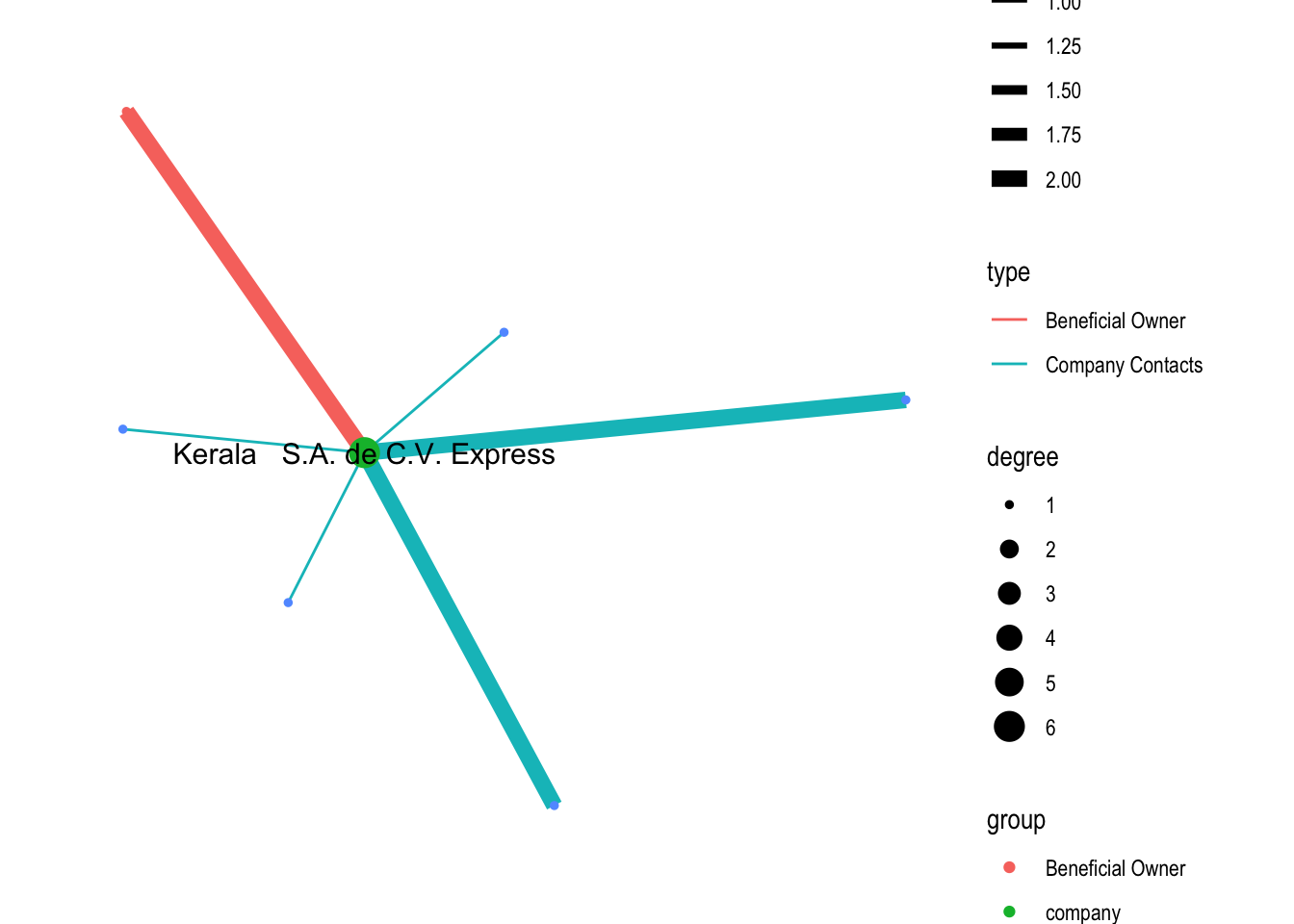
Similar anomalies as previous one.
tidy_nodes <- mc3_nodes %>%
unnest_tokens(word, id, to_lower = TRUE, strip_punct = TRUE,drop = FALSE)# Create a list of custom stopwords that should be added
word <- c("llc","plc","ltd","inc","de","del","company","corporation","liability")
lexicon <- rep("custom", times=length(word))
# Create a dataframe from the two vectors above
mystopwords <- data.frame(word, lexicon)
names(mystopwords) <- c("word", "lexicon")
# Add the dataframe to stop_words df that exists in the library stopwords
stop_words <- dplyr::bind_rows(stop_words, mystopwords)stopwords_removed <- tidy_nodes %>%
anti_join(stop_words) stopwords_removed %>%
count(word, sort = TRUE) %>%
top_n(15) %>%
mutate(word = reorder(word, n)) %>%
ggplot(aes(x = word, y = n)) +
geom_col() +
xlab(NULL) +
coord_flip() +
labs(x = "Unique words of ID",
y = "Count",
title = "Top 15 Count of unique words found in company ID")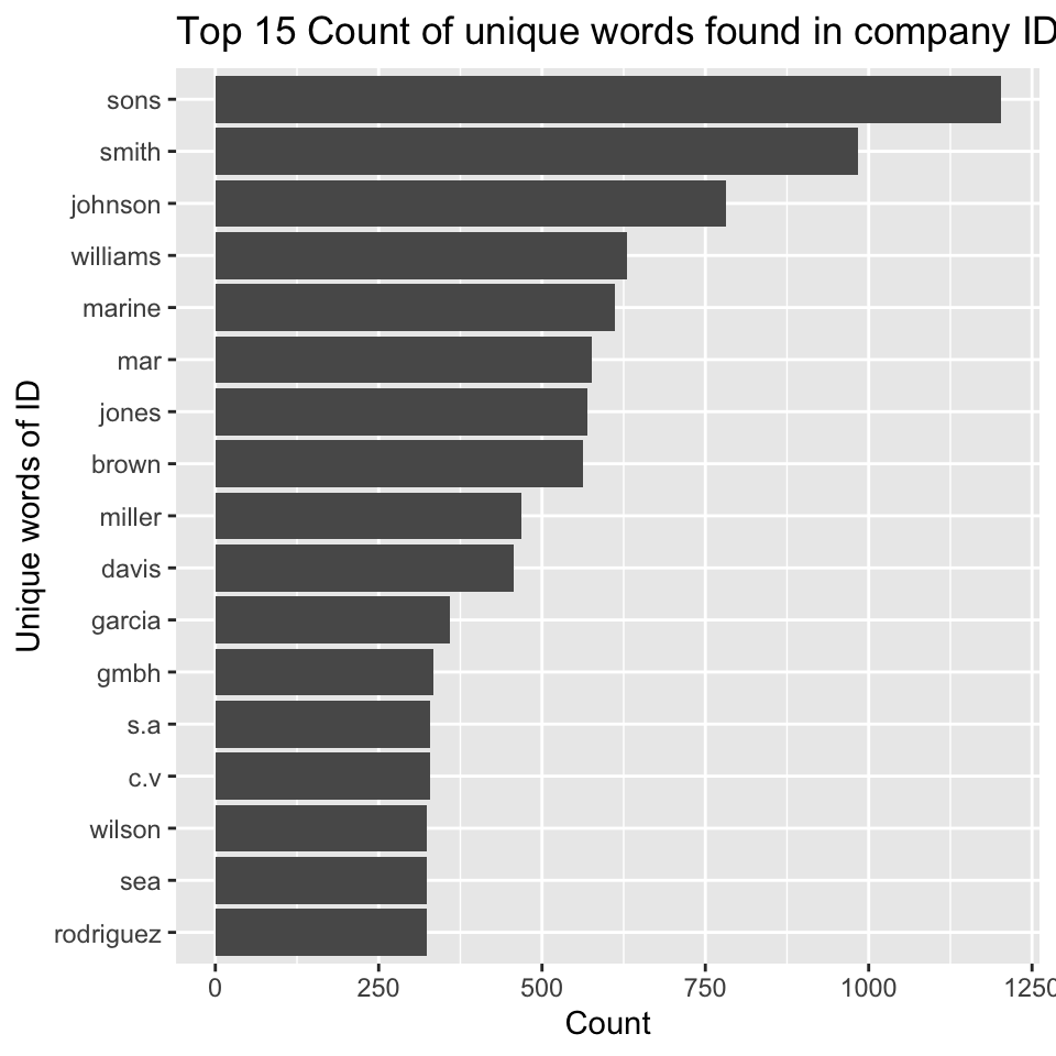
nodes_sons <- mc3_nodes %>%
  filter(type=='Company') %>%
  select("id","country","type","product_services") %>%
  mutate(n_sons = str_count(id, "Sons")) %>%
  filter(n_sons>0) %>%
distinct()edges_sons <- nodes_sons%>%
select(id,country) %>%
distinct() %>%
left_join(mc3_edges,by=join_by(id==source),keep=TRUE,multiple="all") %>%
group_by(source,target,type) %>%
summarise(weight=sum(weight)) %>%
drop_na(weight) %>%
ungroup()nodes_sons_extract <- rbind(edges_sons %>%
rename(id=source)%>%
mutate(group='company') %>%
select(id,group)%>%
distinct(),
edges_sons %>%
rename(id=target) %>%
rename(group=type) %>%
select(id,group) %>%
distinct()) %>%
left_join(mc3_nodes%>%select("id"),
by = 'id', unmatched="drop", keep = FALSE, multiple= 'first')visNetwork(nodes_sons_extract,edges_sons%>%
rename(from=source)%>%
rename(to=target)) %>%
visIgraphLayout(layout = "layout_with_fr") %>%
visEdges(smooth = list(enabled = TRUE,
type = "curvedCW")) %>%
visOptions(highlightNearest = TRUE,
nodesIdSelection = TRUE) %>%
visLegend() %>%
visLayout(randomSeed = 123)Those nodes are individually connected with different set of nodes, and no obvious cluster of company contacts, indicating there’s no intensely close connected group of companies.
nodes_smith <- mc3_nodes %>%
  filter(type=='Company') %>%
  select("id","country","type","product_services") %>%
  mutate(n_sons = str_count(id, "Smith")) %>%
  filter(n_sons>0) %>%
distinct()edges_smith <- nodes_smith%>%
select(id,country) %>%
distinct() %>%
left_join(mc3_edges,by=join_by(id==source),keep=TRUE,multiple="all") %>%
group_by(source,target,type) %>%
summarise(weight=sum(weight)) %>%
drop_na(weight) %>%
ungroup()nodes_smith_extract <- rbind(edges_smith %>%
rename(id=source)%>%
mutate(group='company') %>%
select(id,group)%>%
distinct(),
edges_smith %>%
rename(id=target) %>%
rename(group=type) %>%
select(id,group) %>%
distinct()) %>%
left_join(mc3_nodes%>%select("id"),
by = 'id', unmatched="drop", keep = FALSE, multiple= 'first')visNetwork(nodes_smith_extract,edges_smith%>%
rename(from=source)%>%
rename(to=target)) %>%
visIgraphLayout(layout = "layout_with_fr") %>%
visEdges(smooth = list(enabled = TRUE,
type = "curvedCW")) %>%
visOptions(highlightNearest = TRUE,
nodesIdSelection = TRUE) %>%
visLegend() %>%
visLayout(randomSeed = 123)